

[P15] TabPFN and TabICL for fraud detection - 1
Moving on from toy examples to realistic workflows

This post continues my series on tabular foundation models. So far, I have covered the basic vocabulary of tabular foundation models in P3, the posterior predictive distribution in P4, the architecture in P5, pre-training in P6, the TabPFN repository in P7, the hands-on demo’s classification and regression examples in P8, TabPFN Client in P9, TabPFN embeddings in P10, TabPFN’s predictive behavior in P11, time series forecasting with TabPFN in P12, using TabPFN for causal inference in P13, and comparing TabPFN, TabICL, and supervised ML models in P14.
Yesterday, I created a notebook that brought TabPFN and TabICL into the same supervised-learning examples. That was a useful first comparison, but the examples were still close to toy examples. I later felt that I wanted to move on to examples that are closer to realistic data science workflow as soon as possible.
Today I moved one step in that direction. I built a fraud-detection workflow using TabICL, TabPFN, Logistic Regression, and XGBoost. I am still learning these models by building and running examples, so I treat this notebook as a practical exploration rather than a definitive evaluation. Fraud detection is a useful first workflow because it is widely used. In addition, it is an interesting example from a technical perspective because the positive class is rare, plain accuracy is misleading, and the practical question is not only whether a model has a good score, but whether it produces a usable review queue under runtime, calibration, and deployment constraints.
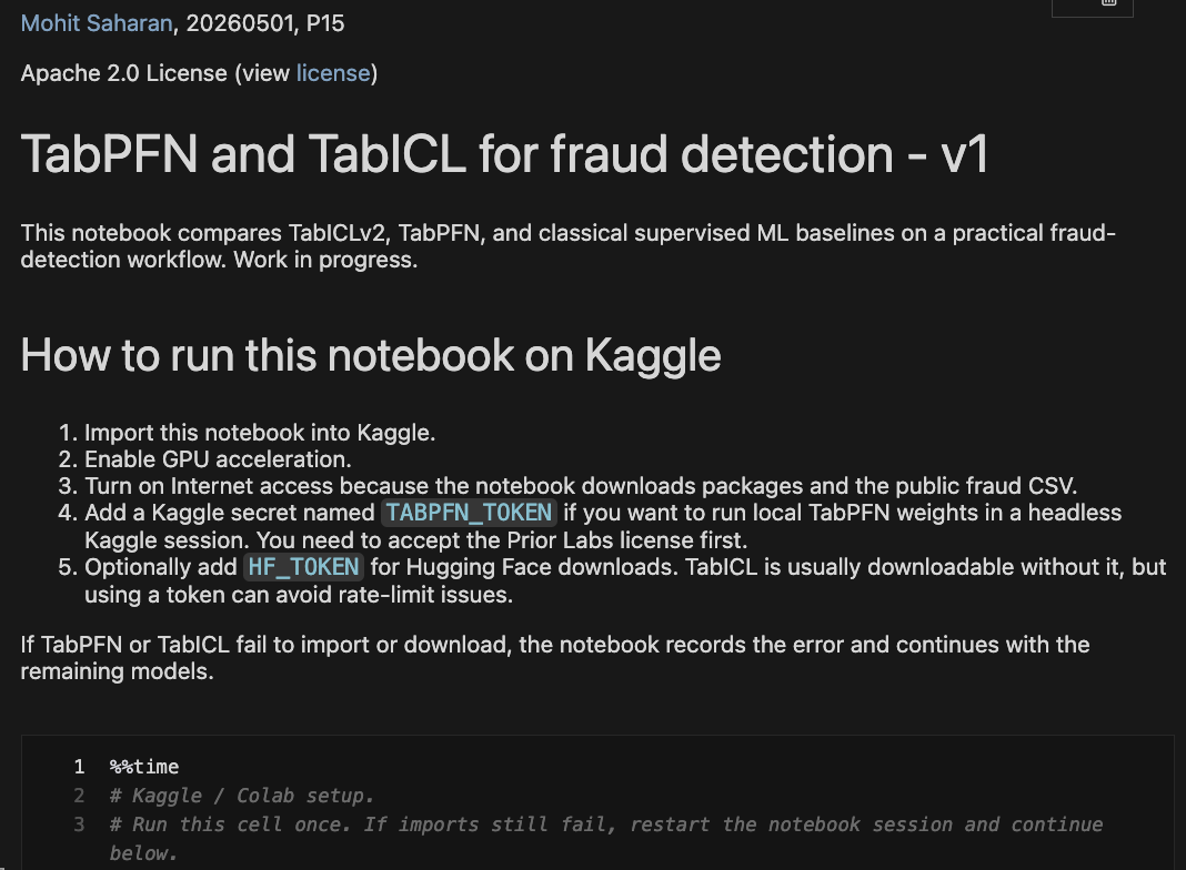
You can find the notebook here on my GitHub repository. As explained in the notebook, it could also be run using time as a model feature (USE_TIME_AS_FEATURE = True) as the only change, and that notebook is available here. The Time=True notebook is a sensitivity check because timestamp-derived behavior can be useful in fraud workflows, but it can also encode period-specific artifacts that need careful production review.
Usually, I write these posts with the conceptual background preceding the work of that day. Today, I am writing this post differently because I have included a lot of conceptual background and interpretation of the results in the notebook. Therefore, the conceptual background given in the following section is meant to supplement that given in the notebook, should the reader need it.
Today’s work is meant to be read directly from the notebook. In future posts, I plan to develop this notebook further to ensure a realistic data science workflow is used by testing it in various ways.
Conceptual Background
Tabular Foundation Models in This Notebook
A tabular foundation model, or TFM, is a pretrained model intended to work across many tabular prediction tasks. In this post, the two TFMs are TabICLv2 and TabPFN.
For a practitioner familiar with supervised ML, the main difference is this: when I call .fit() on Logistic Regression or XGBoost, I am training a task-specific model from the current dataset. When I call .fit() on TabICL or TabPFN in this notebook, I am not training their large pretrained model weights from scratch; I am giving the model labelled rows as task context, and then the model uses that context to predict new rows.
This is why the context set matters for TFMs. The labelled rows given during .fit() are part of the task description the model uses at prediction time. Later in the notebook discussion, I distinguish between the context rows given to TabICL/TabPFN and the holdout rows used for evaluation.
Fraud Detection Is a Rare-Event Ranking Problem
The public credit-card fraud dataset used in the notebook has 284,807 transactions and 492 fraud cases. That is a fraud rate of about 0.17%.
In a dataset like this, accuracy is not a good primary metric by itself, where accuracy is the fraction of all predictions that are correct. A model that predicts “not fraud” for every transaction would be more than 99% accurate, but it would not help a fraud team find fraud cases.
A more relevant question is whether the model can put fraud cases near the top of a ranked list of risky transactions. For that, the useful concepts are precision, recall, and Average Precision.
Precision answers: among the transactions the model flags, what fraction are actually fraud?
Recall answers: among all fraud transactions, what fraction did the model catch?
Average Precision, or AP, summarizes the precision-recall curve across many possible thresholds. Higher AP is better. AP is more informative than accuracy here because it focuses on the rare positive class.
I also report ROC AUC. ROC AUC measures how often the model ranks a random fraud transaction above a random non-fraud transaction. Higher ROC AUC is better. However, I do not use it as the main result because ROC AUC can look good even when the actual fraud review queue still needs separate inspection.
Fraud Teams Deploy Alert Queues, Not Average Precision
Average Precision is useful for comparing rankers, but fraud teams usually do not deploy “Average Precision.” They deploy review queues.
For example, a team might ask:
If we review the top 100 transactions, how many frauds do we catch?
If we can review the top 0.5% of transactions, what is precision and recall?
If we want to catch 80% of fraud cases, how many alerts must we investigate?
If we want to catch 90% of fraud cases, does the review queue become too large?
Here, the phrase “alerts needed to reach 80% recall” means this: sort all transactions by model score from highest risk to lowest risk, then count how many transactions must be reviewed before 80% of the known fraud cases have appeared in that review list. Fewer alerts are better at a fixed recall target. Higher precision is also better because it means fewer false alerts in the review queue.
This is why the notebook includes alert-budget outputs. The goal is not only to ask which model has the highest AP, but also to inspect whether similar AP values lead to different operational outcomes.
Time-Aware Validation Matters
In ordinary tabular ML examples, we often use random train-test splits or random cross-validation. That is often fine for introductory demos, but it is less realistic for fraud detection. Fraud systems care about future transactions. Therefore, model selection should be based on earlier data and evaluation should happen on later data.
The notebook sorts the data by Time and uses four windows:
earliest 60% of transactions: training period;
next 10% of transactions: validation period for classical model selection;
next 10% of transactions: calibration period for probability calibration;
final 20% of transactions: future holdout.
This is still a simplified public-data workflow, but it is closer to a real fraud setting than random cross-validation. This is why the notebook has train, validation, calibration, and final holdout windows rather than one random train-test split.
Calibration Is Different From Ranking
A model can rank fraud cases well while producing poorly calibrated probabilities. This distinction matters.
If a model score is used only to sort transactions into a review queue, ranking quality is the main issue. If a score is interpreted as “this transaction has a 12% fraud probability,” then probability calibration matters.
A calibrated model is a model whose predicted probabilities match observed frequencies reasonably well. For example, among transactions that receive a predicted fraud probability near 10%, roughly 10% should actually be fraud if the model is well calibrated.
In the notebook, the calibrated Logistic Regression and calibrated XGBoost rows are not entirely new model families. They are the selected classical models plus a post-hoc sigmoid calibration step. The sigmoid calibration learns a mapping from the model’s scores to probabilities using the separate calibration window.
The notebook uses two calibration-related metrics:
Brier score: the mean squared error between predicted probabilities and the true 0/1 labels. Lower is better.
Log loss: a probability-sensitive loss that strongly penalizes confident wrong probabilities. Lower is better.
Because the TFM context is sampled differently from the full holdout, I treat probability calibration as something to inspect rather than assume.
Why Compare Against Tuned Classical Baselines?
If I compare TabICL and TabPFN against untuned classical models, the comparison would be weak. In normal data science workflows, a team would tune Logistic Regression or XGBoost, select hyperparameters on validation data, refit the selected model, and check calibration if probabilities are used for decisions.
So the notebook uses:
Logistic Regression as a simple classical baseline.
XGBoost as a widely used boosted-tree baseline.
Calibrated variants of both classical models using a separate calibration window.
TabICLv2 and TabPFN as foundation-model comparators.
I intentionally leave out Random Forest and CatBoost today to avoid leaning toward a broad benchmark. For this workflow test, I use fewer models and spend more space on validation design, full-holdout evaluation, alert-budget analysis, calibration diagnostics, runtime notes, and leakage checks.
Closing thoughts
This is all for today. I will pick it up next week from here. In the meantime, give the notebook a spin in Kaggle and let me know what you think.
Update: the notebook is now available on Kaggle and can be cloned directly. Check out: https://www.kaggle.com/code/msaharan/tabpfn-tabicl-fraud-detection-msaharan-20260501.