

[P26] Architecture of TabICLv2: repeated feature grouping
A technical guide to TabICLv2 repeated feature grouping: why similar columns confuse encoders, how circular shifts add context, with NanoTabICL implementation.

With this post, I am starting a six-part miniseries on the architecture of TabICLv2. The goal is to cover the architecture one subsection at a time, so each post can focus on the details needed to understand that component without making a single article too long. The reference for all posts in this miniseries is the TabICLv2 paper (arXiv). For a hands-on demo, I will use the NanoTabICL implementation as the code companion for this miniseries. It is a short (~170 lines of code) self-contained implementation of the TabICLv2 architecture for educational and experimental purposes. It’s a good point to start before diving into the full model code.
The following figure illustrates the architecture of TabICLv2. This post covers repeated feature grouping. Later posts will cover target-aware embedding, column/row transformers, QASSMax, and the prediction heads.

Repeated feature grouping
Let’s assume a dataset with the following properties and notation:
\(n\) rows and \(m\) columns,
feature random variables denoted as \((X_1,\ldots,X_m),\)
a target random variable denoted as \(Y\),
the value of feature \(j\in\{1,\ldots,m\}\) in row \(i\in\{1,\ldots,n\}\) denoted as \(x_{ij}\), and
the full \(j\)-th column denoted as \(x_{\cdot j}=(x_{1j},\ldots,x_{nj})\).
TabICLv2 first asks how to represent the features in a table.
The problem: similar columns, different roles
In tabular data, two features can have similar marginal distributions,
where \(P_{X_j}\) denotes the marginal distribution of feature \(X_j\). But similar marginals do not imply similar predictive roles. For example, days_since_signup and days_since_last_purchase may both be positive, right-skewed variables, but their relationships to churn can be very different. This creates a representation problem: before the model can reason over feature interactions, its initial feature embeddings must preserve enough information to tell features apart.
Independent column embedding collapses
TabICL-style feature embedding can process each feature with the same encoder. A simplified way to write such an independent column encoder is
where \(d\) is the embedding dimension. The column vector \(x_{\cdot j}\) is mapped to a feature representation
Each column is embedded on its own, without looking at neighboring columns. But if \(\phi\) mostly sees each feature through its own values, then two columns with similar empirical distributions may be mapped to similar embeddings:
Here \(\|\cdot\|_2\) is Euclidean distance and \(\cos(e_a,e_b)\) is cosine similarity. This is the representation-collapse problem: distinct features become nearly indistinguishable in representation space even though their semantics, correlations, or target relationships differ.
The issue here is that the marginal distribution is not the entire identity of a feature. In reality, a feature is also characterized by its joint behavior with other features and with the target. Individual feature embedding can underuse this context. Repeated feature grouping addresses the feature-feature part of that context; the next post covers how target information enters the representation.
Grouping neighboring columns can lead to information loss
TabPFNv2 and TabPFN-2.5 mitigate this collapse by grouping multiple columns into single tokens. But, although grouping gives each feature token some neighboring-feature context, it also reduces the number of effective feature tokens, which can discard fine-grained feature information. The tradeoff is that one token now represents several original columns, so the model has fewer distinct feature positions to work with.
Downstream attention layers then operate on coarser tokens. If fine-grained feature identity is weakened early, later layers have less direct information with which to distinguish individual columns. TabICLv2 uses repeated feature grouping to keep the contextualization benefit while preserving \(m\) effective feature positions.
TabICLv2’s fix: grouping with circular shifts
For a table with \(m\) feature columns, TabICLv2 creates \(m\) groups with \((0,1,3)\) offset pattern relative to every feature with circular shifts. This is why the method is called repeated feature grouping.
To understand this mathematically, let us define the mapper
so \(\rho(t)\) maps any integer \(t\) back into the column index set \(\{1,\ldots,m\}\). Then, the group anchored at feature \(j\) contains columns
For example, for \(m=5\) columns:

Here, feature 1 appears as anchor in group 1, as offset \(+1\) in group 5, and as offset \(+3\) in group 3.

For row \(i\), the grouped input for position \(j\) is
where the vector \(g_j(i)\in\mathbb{R}^3\) contains three scalar feature values from the same row. For example, \(g_1(i)=(x_{i,1},x_{i,2},x_{i,4})\) takes three values from column \(j\), \(j+1\), and \(j+3\) of row \(i\). Each group is encoded by a shared linear map
producing
The resulting tensor \(E_1\in\mathbb{R}^{n\times m\times d}\) contains one \(d\)-dimensional embedding for each row \(i\) and each group position \(j\). Put simply, one shared linear map turns each 3-value group into a \(d\)-dimensional token.
With the shift pattern \((0,1,3)\), for \(m \geq 7\) columns, no pair of columns appears together in more than one group. This gives each feature several contextual views without repeatedly coupling the same feature pairs. The result is a representation that helps prevent feature symmetries between neighboring columns while preserving \(m\) effective feature positions.
Implementation in NanoTabICL
In NanoTabICL, repeated feature grouping happens at the start of NanoTabICLv2.forward. The relevant model parameters are set during initialization:
 self.feature_group_size = feature_group_size
 self.x_embed = nn.Linear(feature_group_size, embed_dim)
The default feature_group_size is 3, so self.x_embed is a shared linear map from a 3-value feature group into the token dimension. This corresponds to the mathematical map
The grouping itself is implemented by indexing shifted versions of the column axis:
 idxs = torch.arange(n_cols, dtype=torch.long, device=x.device)
 x = torch.stack(
     [x[:, :, (idxs + (2 ** i - 1)) % n_cols]
      for i in range(self.feature_group_size)],
     dim=-1,
 )
 emb = self.x_embed(x)
The expression (2 ** i - 1) is the code version of the offset pattern. With feature_group_size=3, the loop uses:
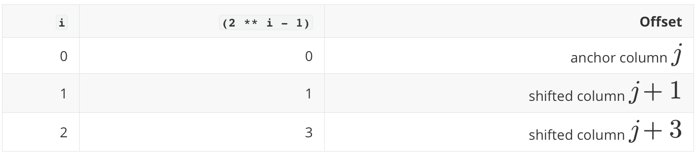
The modulo operation % n_cols is the circular wraparound. If idxs = [0, 1, 2, 3, 4], then the offset 3 gives [3, 4, 0, 1, 2], so the last columns wrap back to the beginning.
The shape transition is the main thing to notice:
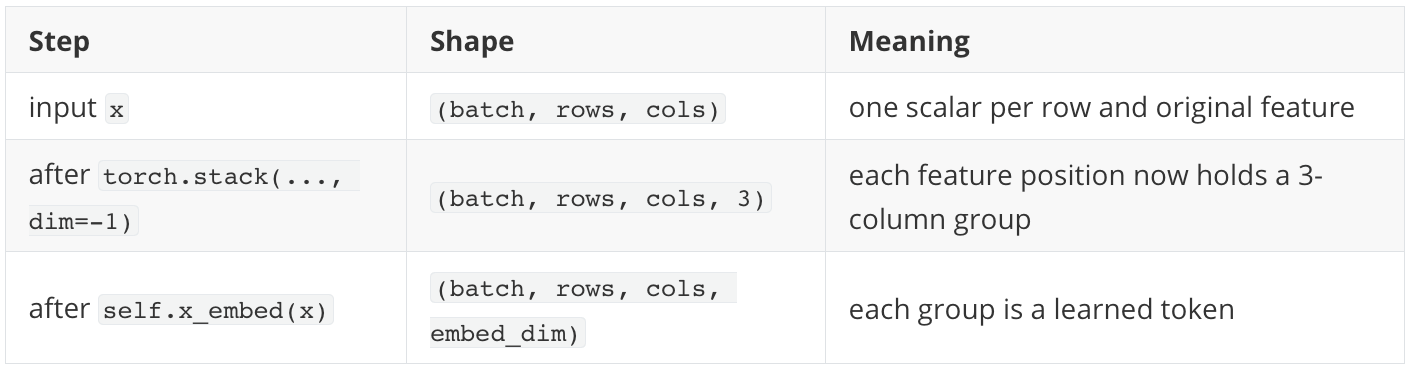
So NanoTabICL keeps the same number of column positions, cols, but each position has already looked at a small circular group of neighboring columns. That is the implementation counterpart of preserving \(m\) effective feature slots while giving each slot local feature context.
Summary
Repeated feature grouping addresses a core weakness of independently embedding tabular features: columns with similar value distributions can become hard to distinguish. TabICLv2 groups each feature with shifted companion features, giving the model multiple contextual views while keeping the number of effective feature positions unchanged. The next post covers target-aware embedding, the step where TabICLv2 injects observed targets into the feature representations of training rows.
thank you! so there is one linear layer that is used to embed all groups at once? why there is in select batch and rows? batch is not used to select rows?