[P27] Architecture of TabICLv2: target-aware embedding

How TabICLv2 uses target-aware embedding to add training labels to tabular in-context learning tokens while preventing label leakage in test rows.

In the previous post, we looked at the first step in TabICLv2’s architecture: repeated feature grouping. That step gives each feature position a small amount of neighboring-column context, helping the model avoid collapsing similar-looking columns into nearly identical representations while still preserving \(m\) effective feature positions.

But repeated feature grouping is still feature-only. It tells the model more about how columns sit next to other columns, but it does not yet tell the model which rows produced which outcomes. The next architectural step, target-aware embedding, adds that supervised signal for training rows.

The following figure shows the full TabICLv2 architecture. This post focuses on the target-aware embedding block, immediately after repeated feature grouping.

TabICLv2 architecture; this post covers target-aware embedding.

In this post, we start from the feature-only tensor \(E_1\), add observed targets only to training-row tokens, and leave test rows unlabeled.

Target-aware embedding

Starting point: feature-only tokens \(E_1\)

Start with the feature matrix after preprocessing/normalization:

\(X=(x_{ij})\in\mathbb{R}^{n\times m},\)

where \(n\) is the number of rows, \(m\) is the number of feature columns, and \(x_{ij}\) is the value of feature \(j\) in row \(i\). In the previous post, repeated feature grouping produced a feature-token tensor

\(E_1\in\mathbb{R}^{n\times m\times d},\)

containing one \(d\)-dimensional embedding for each row \(i\in\{1,\ldots,n\}\) and each group position \(j\in\{1,\ldots,m\}\). The token

\(E_1[i,j]\in\mathbb{R}^d\)

therefore represents row \(i\) at grouped feature position \(j\). At this point the representation is still feature-only. It encodes the input values \(X\), including the local feature context introduced by repeated feature grouping, but it does not yet include the observed targets of the training rows.

The operation: add a target embedding to every training-row token

Target-aware embedding changes \(E_1\) into a target-aware tensor

\(E_2\in\mathbb{R}^{n\times m\times d}\)

by adding an embedding of the observed target \(y_i\) to each feature token in training row \(i\). This is an elementwise vector addition in the same \(d\)-dimensional token space.

To write the operation cleanly, let \(n_\text{train}\) be the number of training rows. In the code implementation, training rows are placed first, so

\(\mathcal{I}_\text{train}=\{1,\ldots,n_\text{train}\}\)

is the set of row indices whose targets are observed. The test rows are

\(\mathcal{I}_\text{test}=\{n_\text{train}+1,\ldots,n\},\)

whose targets must be predicted. For \(i\in\mathcal{I}_\text{train}\), \(y_i\in\mathcal{Y}\) denotes the observed target for row \(i\), where \(\mathcal{Y}\) is the target space. In classification, \(\mathcal{Y}\) is a finite set of class labels; in regression, \(\mathcal{Y}\subseteq\mathbb{R}\).

Define the target-aware embedding map

\(\operatorname{Embed}_\text{TAE}:\mathcal{Y}\rightarrow\mathbb{R}^d.\)

Then define a row-level vector

\(u_i= \begin{cases} \operatorname{Embed}_\text{TAE}(y_i), & i\in \mathcal{I}_\text{train},\\ \mathbf{0}_d, & i\notin \mathcal{I}_\text{train}, \end{cases}\)

where \(\mathbf{0}_d\in\mathbb{R}^d\) is the zero vector. The target-aware representation is

\(E_2[i,j]=E_1[i,j]+u_i, \qquad i=1,\ldots,n,\quad j=1,\ldots,m,\)

where for a training row,

\(E_2[i,j]=E_1[i,j]+\operatorname{Embed}_\text{TAE}(y_i), \qquad i\in\mathcal{I}_\text{train},\)

while for a test row,

\(E_2[i,j]=E_1[i,j], \qquad i\in\mathcal{I}_\text{test}.\)

For each training row \(i\), TabICLv2 computes one target vector and broadcasts it across all \(m\) feature tokens in that row. Test rows receive the zero vector instead. This boundary is essential: for test rows, \(y_i\) is the value the model must infer, so adding \(\operatorname{Embed}_\text{TAE}(y_i)\) would leak the answer.

Classification vs regression implementations

The embedding map depends on the prediction task. For classification, it maps discrete class labels to label vectors; for regression, it maps a scalar target to the token space.

For classification with \(K\leq K_{\max}\) classes, assume labels have been encoded as

\(y_i\in\{0,\ldots,K-1\}.\)

In TabICLv2, \(K_{\max}=10\) for the pretrained small-class target encoder. The embedding map can be viewed as a learned lookup table

\(W_\text{cls}\in\mathbb{R}^{K_{\max}\times d}, \qquad \operatorname{Embed}_\text{TAE}(y_i)=W_\text{cls}[y_i].\)

Here \(W_\text{cls}[k]\in\mathbb{R}^d\) is the target vector associated with class \(k\). The full TabICLv2 implementation realizes this with a one-hot-plus-linear layer, which is equivalent to selecting a learned vector for each supported class. NanoTabICL uses an nn.Embedding wrapper for the same lookup-table idea.

Tasks with more than \(K_{\max}=10\) classes need extra handling. The full TabICLv2 implementation uses mixed-radix ensembling for the target-aware column-embedding stage and hierarchical classification later in the ICL stage. That many-class machinery is outside this post’s small-class view; here we focus on the standard \(K\leq 10\) case.

For regression, where \(y_i\in\mathbb{R}\), the target embedding is a learned linear layer, which can be written as an affine map from the scalar target to the \(d\)-dimensional token space:

\(\operatorname{Embed}_\text{TAE}(y_i)=a y_i+b, \qquad a,b\in\mathbb{R}^d,\)

where \(a\) and \(b\) are learned vectors. In both classification and regression, the output of \(\operatorname{Embed}_\text{TAE}\) lives in \(\mathbb{R}^d\), the same space as the feature token \(E_1[i,j]\). That is why direct addition is well-defined.

Why add to tokens instead of appending a target column?

If the target were appended as a separate token, the feature-token count would change from \(m\) to \(m+1\). Target-aware addition keeps the shape fixed:

\(\text{shape}(E_2)=\text{shape}(E_1)=n\times m\times d.\)

The label information is therefore available at every grouped feature token before the column-wise and row-wise transformer stages, but the architecture still processes \(m\) feature positions rather than \(m+1\). This is different from the TabPFNv2-style target-column appending, where the target is represented as an additional column alongside the feature columns.

Why this helps before the transformers run

Keeping the shape fixed is the computational benefit. The representational benefit connects back to representation collapse, but from a different angle than repeated feature grouping.

The next stage is column-wise processing: for each grouped feature position \(j\), the transformer processes that position across many rows. Because training rows now carry embedded targets, the column-wise transformer can see feature patterns together with observed outcomes.

Let \(Y\) denote the target random variable. In the previous post, we considered two feature random variables \(X_a\) and \(X_b\) with similar marginal distributions,

\(P_{X_a}\approx P_{X_b},\)

where \(P_{X_j}\) denotes the marginal distribution of feature \(X_j\). Similar marginals do not imply similar predictive roles. The two features can still have different target relationships:

\(P(Y\mid X_a=x)\neq P(Y\mid X_b=x)\)

for some values \(x\). Repeated feature grouping helps with the feature-feature part of this problem: a token is not built from one isolated scalar. Target-aware embedding helps with the feature-target part: during column-wise processing, training-row tokens carry both a feature representation and the observed outcome for that row.

The important nuance is that target-aware embedding does not distinguish feature positions within the same row by itself. The same vector \(\operatorname{Embed}_\text{TAE}(y_i)\) is added to every grouped feature token in row \(i\). The feature-position information still comes from \(E_1[i,j]\); the target-aware term supplies row-level supervised context.

This row-level supervised context becomes useful across examples. For training rows \(i\) and \(r\) with different targets,

\(E_2[i,j]-E_1[i,j]=\operatorname{Embed}_\text{TAE}(y_i), \qquad E_2[r,j]-E_1[r,j]=\operatorname{Embed}_\text{TAE}(y_r).\)

So, for each grouped feature position \(j\), the column-wise transformer receives examples of the form “this feature pattern occurred in a row with this target.” Across many rows, that makes feature-target association available earlier than it would be in a purely feature-only embedding.

Informally, for a training row with feature vector \(x_i=(x_{i1},\ldots,x_{im})\), the representation changes from a feature-only encoding to a feature-target encoding:

\(E_1[i,\cdot]\approx \phi(x_i), \qquad E_2[i,\cdot]\approx \psi(x_i,y_i).\)

Here \(E_1[i,\cdot]\) and \(E_2[i,\cdot]\) denote all grouped feature tokens for row \(i\), while \(\phi\) and \(\psi\) are informal names for feature-only and feature-target representation functions. The feature-target encoding applies only to training rows; test rows still carry \(E_1\) at this stage. This is the first target injection in TabICLv2. A second target embedding is added later, after row aggregation, before dataset-wise ICL.

Implementation in NanoTabICL

NanoTabICL implements target-aware embedding with two pieces: a task-dependent target embedder and one masked in-place addition to the training rows.

During initialization, the target embedder depends on whether the model is configured for classification or regression:

self.y_embed_in = (
    ClassEmbedding(max_classes, embed_dim)
    if max_classes > 0
    else nn.Linear(1, embed_dim)
)

For classification, ClassEmbedding is a learnable lookup table:

class ClassEmbedding(nn.Embedding):
    def reset_parameters(self) -> None:
        nn.init.uniform_(self.weight, -1/math.sqrt(self.num_embeddings), 1/math.sqrt(self.num_embeddings))

    def forward(self, y: torch.Tensor) -> torch.Tensor:
        return super().forward(y.squeeze(-1).long())

The call to long() turns labels such as 0, 1, or 2 into embedding-table indices. The custom initialization matches the nn.Linear weight initialization scale. For regression, nn.Linear(1, embed_dim) implements the affine scalar-to-vector map \(a y_i+b\).

The actual target-aware update is one line in forward:

emb[:, :n_train] += self.y_embed_in(y[:, :, None, None])

The shape logic is the key to reading this line:

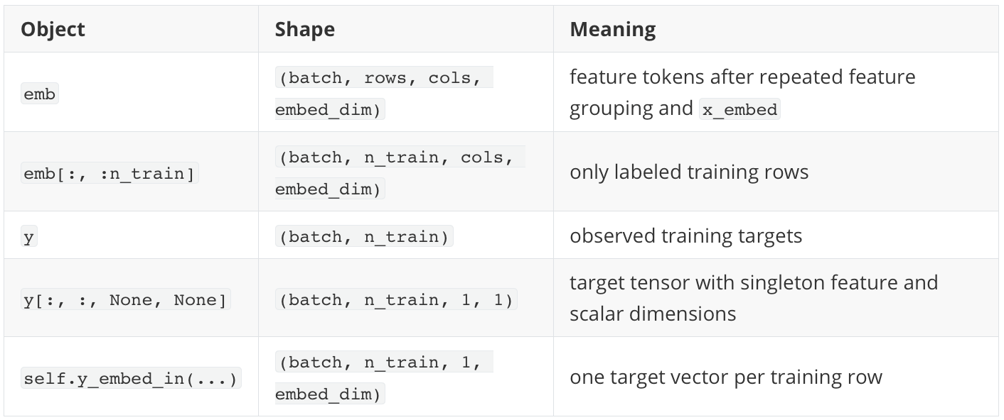
PyTorch broadcasting adds that target vector across all cols grouped feature positions in the corresponding training row. This is the code version of:

\(E_2[i,j]=E_1[i,j]+\operatorname{Embed}_\text{TAE}(y_i), \qquad i\in\mathcal{I}_\text{train}.\)

The masking boundary is the important safety rule. NanoTabICL never indexes emb[:, n_train:] in this addition, so test rows remain feature-only at this stage:

training rows: feature token + target embedding
test rows:     feature token only

That single slice, :n_train, is what prevents target leakage in the implementation.

Summary

After target-aware embedding, training-row feature tokens carry supervised context, while test-row feature tokens remain unlabeled. TabICLv2 gets this effect by adding one target embedding to every grouped feature token in each labeled row, without changing the \(n\times m\times d\) tensor shape produced by repeated feature grouping.

The result is \(E_2\): a target-aware feature-token tensor ready for the compression-then-ICL pipeline. The next post covers how TabICLv2 compresses these tokens into row representations, adds target information again at the row-token level for labeled rows, and then performs dataset-wise in-context learning.