

[P31] Architecture of TabICLv2: quantile predictions for regression
How TabICLv2 models regression with 999 conditional quantiles, pinball loss, and distribution reconstruction.

This is the last post in the miniseries on the architecture of TabICLv2. The previous post covered many-class classification: how TabICLv2 decomposes large label spaces on both the target-aware embedding side and the ICL output side while keeping the native small-class interface learned during pretraining. This post covers quantile predictions for regression: how TabICLv2 models a continuous target as 999 conditional quantiles.
The TabICLv2 regression head does not directly emit a single point estimate. In a dedicated regression checkpoint trained with pinball loss, it predicts 999 conditional quantiles at probability levels \(\mathcal{A}=\{0.001,0.002,\ldots,0.999\}\), forming a dense grid that approximates the conditional distribution of the target.
Like classification, regression keeps the same overall backbone structure: repeated feature grouping, target-aware embedding, and the column/row/ICL transformer blocks \(\text{TF}_\text{col}\), \(\text{TF}_\text{row}\), and \(\text{TF}_\text{icl}\); observed targets still enter twice. Classification embeds those targets as class IDs and emits class logits. Regression swaps the task-specific interfaces and loss: scalar linear target embedders replace class lookup tables, and the output MLP emits 999 raw quantiles per test row instead of logits. Its checkpoint also uses bias-free LayerNorm, whereas the classification checkpoint uses LayerNorm with bias.
This post explains what those quantiles represent, how pinball loss trains them, how inference turns the raw grid into a monotone predictive distribution, and how the same outputs support both fast point estimates and probabilistic predictions. It also maps the regression path in NanoTabICL through max_classes=0 and out_dim=999, and notes what the compact model leaves outside the forward pass. The following figure shows the architecture of TabICLv2.
A short quiz at the end lets you check your understanding.
.")
Quantile predictions for regression
Tabular foundation models adopt different strategies for regression. TabPFNv2 and TabPFN-2.5 model the predictive distribution by discretizing the target space into bins and applying cross-entropy loss. TabICLv2 instead uses a dedicated regression checkpoint that directly predicts quantiles. It retains the same overall backbone structure while changing the task-specific interfaces, loss, and LayerNorm configuration.
The subsections below build from quantile definitions and pinball loss to training and inference.
What quantiles are
To see what this regression head is learning, first recall what a quantile represents: the smallest value at which the cumulative probability reaches at least \(\alpha\). Start with the unconditional case: one target \(Y\), no features yet. Let \(Y\) be a real-valued target random variable with cumulative distribution function (CDF)
For a probability level \(\alpha\in(0,1)\), define its quantile function as the generalized inverse
In words, \(Q(\alpha)\) is the smallest target value whose cumulative probability reaches at least \(\alpha\). This definition remains valid when the CDF has jumps. When the CDF is continuous and strictly increasing, it reduces to the familiar inverse relation \(F_Y(Q(\alpha))=\alpha\). For example, \(Q(0.5)\) is the median and \(Q(0.9)\) is the 90th percentile.
Now make the distribution depend on the row. In supervised regression, the target distribution depends on the input row. To avoid overloading the table symbol \(X\), write \(Z\) for the random feature vector of a single row and \(x\) for a particular observed row. The conditional quantile function (CQF) is
Here \(F_{Y\mid Z=x}(q)=P(Y\leq q\mid Z=x)\) is the conditional CDF at row \(x\). The probability level \(\alpha\) selects a location on that row’s conditional distribution. The two notations denote the same quantity, written two ways: \(Q_x(\alpha)\) treats the quantile as a function of \(\alpha\) (the inverse-CDF view, as with \(Q(\alpha)\) above), while \(q_\alpha(x)\) treats \(\alpha\) as a label on the \(\alpha\)-quantile as a function of row \(x\) (the prediction view, as with \(\hat{q}_\alpha(x)\) below). This post uses whichever notation reads more naturally in context.
Instead of asking the model for one conditional summary, TabICLv2 asks it for many summaries spread across the distribution. Specifically, it predicts 999 such quantiles at probability levels
These 999 outputs form a dense grid of estimated points on \(Q_x(\alpha)\). They are not, by themselves, a full predictive distribution; the inference-time distribution wrapper constructs one by making the grid monotone, interpolating between its points, and extrapolating beyond its endpoints.
Pinball loss
Each output is trained with pinball loss, also called quantile loss or check loss. If the model predicts \(\hat{q}_\alpha(x)\) for level \(\alpha\) and the observed target is \(y\), define the residual
The pinball loss is
Equivalently,
Here \(\hat{q}\) is shorthand for \(\hat{q}_\alpha(x)\), and \(\mathbf{1}\{y<\hat{q}\}\) is an indicator. Underprediction means \(y>\hat{q}\), so the loss grows at rate \(\alpha\) as the miss increases. Overprediction means \(y<\hat{q}\), so it grows at rate \(1-\alpha\). The result is a tilted absolute-value penalty.
: asymmetric slopes penalize under- and over-prediction differently.")
This asymmetry makes the loss target a specific quantile. For \(\alpha=0.5\),
so minimizing the expected loss recovers a median. For \(\alpha=0.9\), an equally sized underprediction costs nine times as much as an overprediction. The optimum is therefore pushed upward until it represents the conditional 90th percentile.
Training and constructing a distribution
With pinball loss defined, the regression head trains one raw scalar \(\hat{q}_\alpha(x)\) per level in \(\mathcal{A}\). Each level has a separate output coordinate, but all levels share the backbone and output MLP hidden representation. For each example \((x,y)\), training averages pinball loss equally across all 999 levels:
Predicting each level separately raises one practical issue: the architecture imposes no explicit monotonicity or cross-quantile constraint, and pretraining adds no auxiliary penalty for crossing quantiles. The raw outputs can therefore violate the ordering required of a valid quantile function:
TabICLv2 resolves this issue while turning the grid points into a full predictive distribution at inference. First, it enforces monotonicity (default: sort; alternative: isotonic regression). Second, it piecewise-linearly interpolates between the corrected points. Third, because the grid stops at \(0.001\) and \(0.999\), it extrapolates parametric tails—exponential by default, GPD optional. The reconstructed distribution then exposes a PDF, CDF, inverse CDF (ICDF), and analytical moments across \(\mathbb{R}\).
Prediction intervals and point estimates
Two standard uses of the corrected quantile function are interval construction and point estimation.
Once the raw outputs have been turned into a monotone quantile function, prediction intervals are a direct use of it. Continuing to write \(\hat{q}_\alpha(x)\) for the corrected quantile value, a central \((1-\gamma)\) prediction interval—where \(\gamma\in(0,1)\) is the total tail probability outside the interval—is

For example, a 90% interval uses \(\gamma=0.1\):
If the interval has calibrated marginal coverage—that is, empirically, the fraction of held-out targets falling inside it is close to the nominal level (e.g. ~90%)—it should contain the true target approximately 90% of the time over repeated samples from the same data-generating process. This marginal coverage does not by itself guarantee conditional coverage for every input row or calibration of every individual quantile. It is an empirical calibration property of the predictions, not something guaranteed merely by using pinball loss or by sorting the quantiles.
Prediction intervals use specific quantile levels; point estimation uses the full grid. For point estimation, TabICLv2’s fast mean path averages the 999 predicted quantiles. This is motivated by the quantile-function identity
when the conditional expectation exists. With a dense, evenly spaced grid of quantiles, this integral can be approximated by a simple average. Because \(\mathcal{A}\) is an evenly spaced grid on \((0,1)\), the sum is a Riemann-sum approximation of the integral:
Here \(\hat{\mu}(x)\) is the fast point prediction and \(|\mathcal{A}|=999\). The grid omits \(\alpha=0\) and \(\alpha=1\); the fast mean therefore uses only the \(0.001\)–\(0.999\) grid and ignores the parametric tails extrapolated beyond those endpoints (see the distribution-construction steps above).
The current implementation constructs the monotone distribution before taking this average. Default sorting only reorders values, so it preserves the average of the raw outputs. The current unweighted isotonic-regression alternative can change individual values, but its pooled averages preserve the total sum and therefore the overall average. Monotonicity correction matters for interpreting the outputs as a quantile function and for distribution operations, but neither current correction method changes the simple average.
The same 999 raw outputs therefore support two inference paths: a fast point estimate through averaging, and richer probabilistic predictions through a reconstructed monotone distribution.
Implementation in NanoTabICL
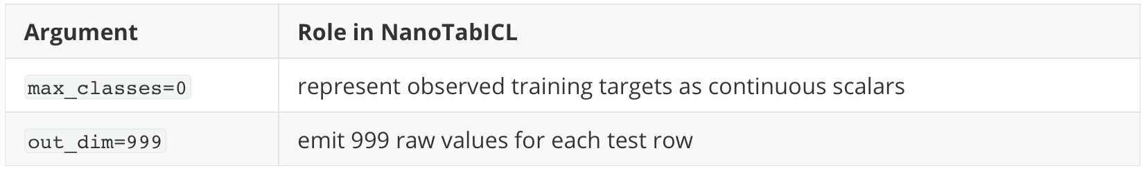
The subsections above describe full TabICLv2 regression inference. NanoTabICL exposes only the regression forward path through max_classes=0 and out_dim=999. The following sections trace the target embedders and output head, explain target scaling, and identify the full TabICLv2 inference steps left outside the compact model.
These two NanoTabICL constructor arguments make the regression path visible:
def __init__(self, max_classes: int, out_dim: int, ...):
    # classification: max_classes = out_dim (= 10 typically)
    # regression: max_classes = 0, out_dim = n_quantiles
The README combines these regression settings in its example:
model = NanoTabICLv2(
    max_classes=0,
    out_dim=999,
    embed_dim=96,
    col_num_blocks=2,
    row_num_blocks=2,
    icl_num_blocks=4,
    col_nhead=4,
    row_nhead=4,
    icl_nhead=4,
)
y_train = torch.randn(batch_size, n_train)
y_test_pred_quantiles = model(X_train_and_test, y_train)
This example instantiates a randomly initialized model. Its 999 outputs acquire quantile meaning only after compatible pinball-loss pretraining or after loading compatible trained regression weights; NanoTabICL provides neither.
These arguments control different sides of the model:
NanoTabICL exposes out_dim directly. The full TabICLv2 constructor instead exposes num_quantiles and internally sets out_dim=num_quantiles for regression.
One more checkpoint-compatibility difference matters: NanoTabICL uses LayerNorm with bias, matching the TabICLv2 classification checkpoint, while the full regression checkpoint uses LayerNorm without bias. The compact model therefore explains the regression architecture, but it is not a drop-in reimplementation of every regression-checkpoint detail.
Regression target embeddings
The task switch appears first in the two target embedders:
self.y_embed_in = (
    ClassEmbedding(max_classes, embed_dim)
    if max_classes > 0
    else nn.Linear(1, embed_dim)
)
self.y_embed_icl = (
    ClassEmbedding(max_classes, icl_dim)
    if max_classes > 0
    else nn.Linear(1, icl_dim)
)
For classification, ClassEmbedding treats each target as an integer class id. For regression, nn.Linear(1, ...) treats each target as one continuous scalar and projects it into the required token space:
y_train scalar
    -> nn.Linear(1, embed_dim)  for feature-token target-aware embedding
    -> nn.Linear(1, icl_dim)    for row-token ICL embedding
The first projection is added before column-wise processing:
emb = self.x_embed(x)
emb[:, :n_train] += self.y_embed_in(y[:, :, None, None])
Here y has shape (batch, n_train). Adding two singleton dimensions gives (batch, n_train, 1, 1). The linear layer transforms the final size-one dimension, producing (batch, n_train, 1, embed_dim), which broadcasts across all grouped feature positions in each training row:
feature-level target embedding:
(batch, n_train)
    -> (batch, n_train, 1, 1)
    -> (batch, n_train, 1, embed_dim)
    -> broadcast across cols
After row compression, the second projection is added before dataset-wise ICL:
emb[:, :n_train] += self.y_embed_icl(y[:, :, None])At this point emb has shape (batch, rows, icl_dim). The added singleton dimension lets nn.Linear(1, icl_dim) produce one row-level target vector for each labeled training row:
row-level target embedding:
(batch, n_train)
    -> (batch, n_train, 1)
    -> (batch, n_train, icl_dim)
Both additions select emb[:, :n_train], so no target value is injected into test rows.
Because both embedders consume raw scalar targets, y_train must be standardized before the forward pass and predictions back-transformed afterward. NanoTabICL scales X_train_and_test internally using training rows, but it does not transform y_train; its feature scaling is also asymmetric because it divides by the training-row standard deviation without subtracting the training mean. The README warns:
# warning: for regression, you need to standardize y yourself
# (and backtransform the output)
This matters because the same standardized target values are passed into both regression target embedders, and the 999 outputs are produced on that standardized scale. Quantiles are equivariant under positive affine maps: if \(Y’ = aY + b\) with \(a>0\), then \(Q_{Y’}(\alpha) = a\,Q_Y(\alpha) + b\). Standardizing and back-transforming therefore preserves each output’s probability-level meaning.
A minimal per-table target transformation would look like:
y_mean = y_train.mean(dim=1, keepdim=True)
y_std = y_train.std(dim=1, unbiased=False, keepdim=True).clamp_min(1e-8)

y_train_scaled = (y_train - y_mean) / y_std
q_scaled = model(X_train_and_test, y_train_scaled)
q_original = q_scaled * y_std[:, :, None] + y_mean[:, :, None]
Every predicted quantile uses the same inverse affine transformation shown above. Target standardization is entirely your responsibility.
From test-row states to raw quantiles
The final ICL block uses labeled training rows as keys and values, while computing outputs only for test-row queries:
emb = self.icl_blocks[-1](emb[:, n_train:], emb[:, :n_train])Its output has shape (batch, n_test, icl_dim). The output head then maps each test-row state to out_dim values:
self.out_mlp = get_mlp(icl_dim, icl_dim * 2, out_dim)
return self.out_mlp(self.out_ln(emb))
after final ICL block: (batch, n_test, icl_dim)
after output MLP: (batch, n_test, out_dim)
with out_dim=999: (batch, n_test, 999)There is no softmax, sorting operation, or monotonicity constraint in this output path. The architecture itself also does not attach \(\alpha\) values to the 999 output positions. Their interpretation as the indexed grid
comes from training each position against its corresponding pinball-loss level. NanoTabICL provides the architecture and raw forward-pass outputs, but it does not provide that pretraining loop.
What NanoTabICL leaves outside the model
NanoTabICL returns the raw tensor (batch, n_test, 999) directly. To make those outputs meaningful quantile predictions, the model must first be trained with the corresponding pinball-loss levels or supplied compatible trained weights. Distribution construction and prediction intervals are then implemented downstream of the tensor. Beyond the forward pass described above, NanoTabICL does not include:
pinball-loss pretraining;
the mapping from output positions to quantile levels as a model object;
monotonicity correction for crossing quantiles;
interpolation, tail extrapolation, or distribution statistics;
a scikit-learn prediction interface.
Summary
TabICLv2 handles regression through a dedicated regression checkpoint that predicts 999 conditional quantiles rather than a single point or a discretized target distribution. Each output level is trained with pinball loss, which targets the corresponding conditional quantile through its asymmetric penalty on under- and over-prediction. The raw 999 scalars are not, by themselves, a valid predictive distribution; at inference time, TabICLv2 sorts or otherwise corrects crossing quantiles, interpolates between grid points, and extrapolates the tails to build a full distribution wrapper.
The same quantile grid supports two inference paths. A fast point estimate averages the 999 predicted levels, approximating the conditional mean through the quantile-function identity. Richer probabilistic outputs come from the reconstructed distribution: central \((1-\gamma)\) prediction intervals read directly from symmetric quantile pairs, where \(\gamma\) is the total tail probability outside the interval, while PDF, CDF, and moment calculations use the interpolated body and parametric tails. Nominal interval coverage is an empirical calibration property, not something guaranteed by pinball loss alone.
Regression reuses the same overall compression-then-ICL backbone structure as classification, while changing the task-specific interfaces, loss, and LayerNorm configuration. Observed training targets are embedded as continuous scalars through linear maps at both the feature-token and row-token stages, and the output head emits out_dim=999 raw values per test row with no softmax or built-in monotonicity constraint. NanoTabICL makes this path visible through max_classes=0 and out_dim=999, but users must standardize y themselves, train the model with the corresponding pinball-loss levels or supply compatible trained weights, and apply the full TabICLv2 inference pipeline downstream of its raw (batch, n_test, 999) output; it leaves pinball-loss pretraining, monotonicity correction, distribution construction, and scikit-learn wrappers outside the model.
This regression path completes the six-part walkthrough of TabICLv2’s architecture: repeated feature grouping, target-aware embedding, compression-then-ICL, QASSMax, many-class classification, and quantile regression. Together, the posts trace one table from grouped feature tokens through row-level in-context learning to either class probabilities or a full predictive distribution over a continuous target.
Quiz
Take the quiz below to test your understanding, and share your answers and doubts in the comments. The questions get progressively harder from 1 to 10.
What does the quantile grid \(\mathcal{A}=\{0.001,0.002,\ldots,0.999\}\) represent?
What is pinball loss, and how does its asymmetry target a specific quantile?
Why are the raw 999 model outputs not, by themselves, a full predictive distribution?
How is pinball loss applied during training for the 999 quantile outputs?
Why can the raw 999 quantile outputs cross, and how does TabICLv2 correct them at inference time?
After monotonicity correction, how does TabICLv2 construct a full predictive distribution from the corrected quantile grid?
How is a central \((1-\gamma)\) prediction interval read from the corrected quantile function, and does pinball loss alone guarantee that a nominal 90% interval covers 90% of held-out targets?
How does TabICLv2’s fast point-estimate path approximate the conditional mean, and why do the current monotonicity-correction methods preserve that mean?
How does TabICLv2’s regression strategy differ from TabPFNv2 and TabPFN-2.5, and which NanoTabICL arguments activate its regression path?
Suppose you only need a fast point estimate and never use prediction intervals, PDF, CDF, or moments. Which inference steps could you skip, and what would you lose?